Getting Started Tutorials
To learn to use BAGLE models, make microlensing events, and make photometric or astrometric plots, we have created an Intro Jupyter Notebook. tutorial. A subset of the content is reproduced below.
Using BAGLE
To make microlensing models:
from bagle import model
from bagle import plot_models
To fit microlensing data with models:
from bagle import model_fitter
Making a PSPL Model with No Parallax
The first step in the tutorial is to generate a PSPL model with no parallax and to use the model to:
Get amplification of event over time
Plot the astrometric shift over time
Animate the microlensing event
First, define a microlensing event with a set of parameters:
mL = 10.0                       # lens mass in Msun
t0 = 57000.00                   # closest approach time in MJD (days)
xS0 = np.array([0.000, 0.000])  # arcsec, arbitrary
beta = 1.4                      # source-lens separation in mas
muS = np.array([8.0, 0.0])      # source proper motion in mas/yr
muL = np.array([0.00, 0.00])    # lens proper motion in mas/yr
dS = 8000.0                     # source distance in pc
dL = 4000.0                     # lens distance in pc
b_sff = [1.0]                   # list of source flux fractions,
                                # one for each filter,
                                # [flux_S / (flux_S + flux_L + flux_N)]
mag_src = [19.0]                # list of source baseline magnitude
                                # one for each filter

event1 = model.PSPL_PhotAstrom_noPar_Param1(mL, t0, beta, dL,
                                            dL / dS, xS0[0], xS0[1],
                                            muL[0], muL[1], muS[0],
                                            muS[1],
                                            b_sff, mag_src)
Note that BAGLE mas many different parameterizations that all
specify the same event. We have chosen Param1.
Once you have created the event, you can see numerous event properties. BAGLE defines event parameteres in heliocentric coordinates unless otherwise specified. To see properties, use:
print(event1.t0)      # Time of closest apparent approach
print(event1.u0_amp)  # Distance apart at t0
print(event1.muRel)   # Source - Lens relative proper motion
You can also evaluate what is happening with the event at different times. Make a time array of 1000 days centered around the event peak:
import numpy as np
t = np.arange(event1.t0 - 500, event1.t0 + 500, 1)
Many functions allow you to get the photometry or astrometry at this list of times:
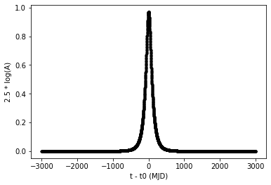
A = event1.get_amplification(t)
dt = t - event1.t0
plt.figure()
plt.plot(dt, 2.5 * np.log10(A), 'k-')
plt.xlabel('t - t0 (MJD)')
plt.ylabel('2.5 * log(A)')
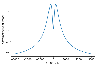
plt.figure()
plt.plot(dt, shift_amp)
plt.xlabel('t - t0 (MJD)')
plt.ylabel('Astrometric Shift (mas)')
The resulting figures are shown below.
- Other methods that return event values over time include:
event1.get_amplificationevent1.get_photometryevent1.get_centroid_shiftevent1.get_astrometryevent1.get_astrometry_unlensedevent1.get_lens_astrometryevent1.get_resolved_shiftevent1.get_resolved_amplificationevent1.get_resolved_astrometry
Making a PSPL Model with Parallax
The second step is to generate a PSPL model with parallax adding the ra (right ascention of lens) and dec (declination of lens). Again, all of the parameters are specified in heliocentric coordinates.
ra = 269.9441667    # in decimal degrees
dec = -28.6449444   # in decimal degrees
mL = 10.0           # lens mass in Msun
t0 = 55150.0        # closest apparent approach time in MJD
xS0 = [0, 0]        # position of source at t0, arbitrary (arcsec)
beta = -2.0         # source - lens separation in mas,
                    # sign follows Gould convention.
muS = [5, 0]        # source proper motion in mas/yr
muL = [0, 0]        # lens proper motion in mas/yr
dS = 8000           # source distance in pc
dL = 4000           # lens distance in pc
b_sff = [1.0]       # list of source flux fractions,
                    # one for each filter,
                    # [flux_S / (flux_S + flux_L + flux_N)]
mag_src = [19.0]    # list of source baseline magnitude
                    # one for each filter

event2 = model.PSPL_PhotAstrom_Par_Param1(mL, t0, beta, dL, dL/dS,
                                          xS0[0], xS0[1],
                                          muL[0], muL[1],
                                          muS[0], muS[1],
                                          b_sff, mag_src,
                                          raL=ra, decL=dec)

print('tE = ', event2.tE)
print('thetaE = ', event2.thetaE_amp)
print('piE = ', event2.piE_amp)
Advanced Astrometric Plots
We demonstrate more advanced astrometric plotting using an example event from Belokurov and Evans 2002. First, define the event:
mL = 0.5  # msun
t0 = 57160.00
xS0 = np.array([0.000, 0.000])
beta = -7.41  # mas
muS = np.array([-2.0, 7.0])
muL = np.array([90.00, -24.71])
dL = 150.0
dS = 1500.0
b_sff = [1.0]
mag_src = [19.0]

belukurov = model.PSPL_PhotAstrom_noPar_Param1(mL, t0, beta,
                                               dL, dL / dS,
                                               xS0[0], xS0[1],
                                               muL[0], muL[1],
                                               muS[0], muS[1],
                                               b_sff, mag_src)
Get the astrometry for the actual lens, actual source, and apparent shifted source position over time:
# Set time range for event
t = np.arange(belukurov.t0 - 3000, belukurov.t0 + 3000, 1)
dt = t - belukurov.t0

# Get lens-induced astrometric shift from centroid for all images
shift = belukurov.get_centroid_shift(t)
shift_amp = np.linalg.norm(shift, axis=1)

# Positions for lens, source, and observed image
lens_pos = belukurov.xL0 + np.outer(dt / model.days_per_year, belukurov.muL) * 1e-3
srce_pos = belukurov.xS0 + np.outer(dt / model.days_per_year, belukurov.muS) * 1e-3
imag_pos = srce_pos + (shift * 1e-3)
Note that the returned quantities (e.g. lens_pos) have dimensions
of [len(t), 2] where the 2 entries represent the R.A. and
Dec. over time. Above, we could have also used:
lens_pos = belukurov.get_lens_astrometry(t)     # lens
srce_pos = belukurov.get_astrometry_unlensed(t) # source, unlensed
imag_pos = belukurov.get_astrometry(t)          # source, micro-lensed
Now make a plot showing where everything is on the sky:
plt.figure()
plt.plot(lens_pos[:, 0], lens_pos[:, 1], 'r--', mfc='none', mec='red')
plt.plot(srce_pos[:, 0], srce_pos[:, 1], 'b--', mfc='none', mec='blue')
plt.plot(imag_pos[:, 0], imag_pos[:, 1], 'b-') #solid blue line
lim = 0.005
plt.xlim(lim, -lim)  # arcsec
plt.ylim(-lim, lim)
plt.xlabel('dRA (arcsec)')
plt.ylabel('dDec (arcsec)')

and the decomposed shifts in x, y, and total amplitude over time where the time is normalized by the Einstein crossing time and the shifts are normalized by the Einstein radius:
f, (ax1, ax2, ax3) = plt.subplots(3, sharex=True)
f.subplots_adjust(hspace=0)
ax1.plot(dt / belukurov.tE, shift[:, 0] / belukurov.thetaE_amp, 'k-')
ax2.plot(dt / belukurov.tE, shift[:, 1] / belukurov.thetaE_amp, 'k-')
ax3.plot(dt / belukurov.tE, shift_amp / belukurov.thetaE_amp, 'k-')
ax3.set_xlabel('(t - t0) / tE)')
ax1.set_ylabel(r'dX / $\theta_E$')
ax2.set_ylabel(r'dY / $\theta_E$')
ax3.set_ylabel(r'dT / $\theta_E$')
ax1.set_ylim(-0.4, 0.4)
ax2.set_ylim(-0.4, 0.4)
ax3.set_ylim(0, 0.4)
